
Illustrated operator examples
Three workflows from recording to saved evidence.
Follow real application views to save a spectrogram, analyse a calibrated dolphin recording, or plan propagation coverage for a sea trial.
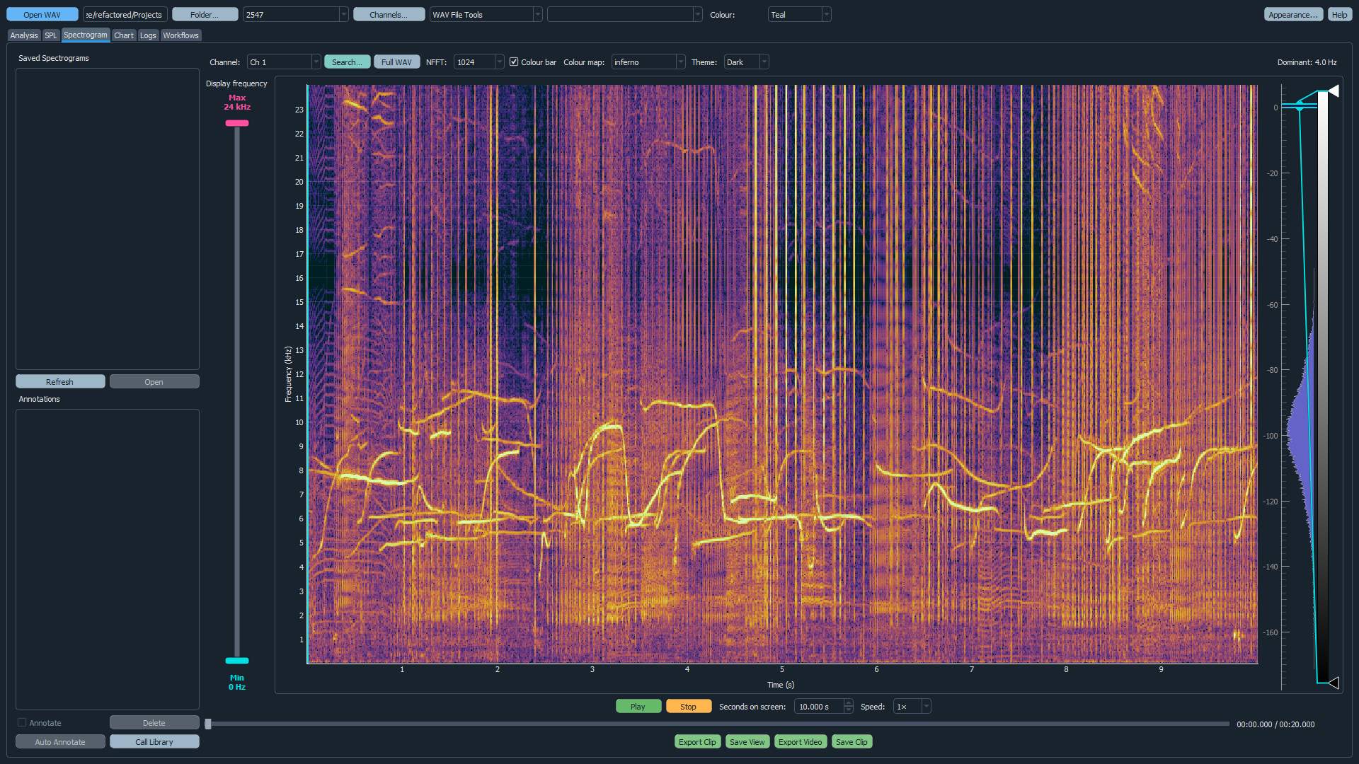
Start with the spectrogram workflow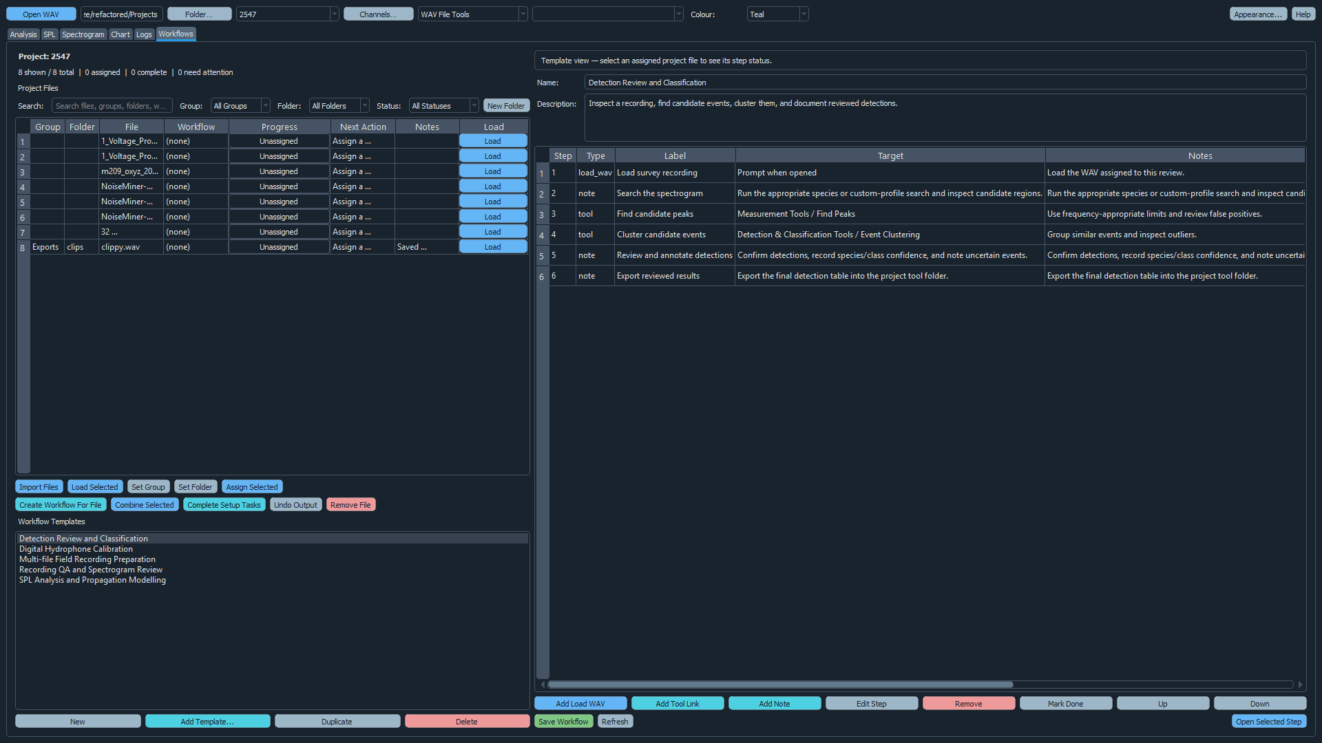
Workflow 01
Generate a spectrogram and save the view.
Result: a traceable PNG in the selected project's spectrograms folder.
- Create or select a project, then open the WAV recording.
- Open Channels, enable and name the channel, and choose OK.
- Open Spectrogram. Select channel, NFFT, colourbar, colourmap, theme, and colour.
- Set Seconds on screen, or choose Full WAV. Adjust the dual-handle frequency range.
- Choose Generate, then use Play and the time slider to locate the signal. Ctrl-drag when a precise region is required.
- Choose Save View, accept or edit the suggested filename, and save.
- Open the PNG and verify that time, frequency, colour scale, channel, and signal are legible.
Resolution check: a larger NFFT improves frequency resolution; a smaller NFFT improves time resolution. Choose settings that preserve the event you need to show.
Workflow 02
Analyse dolphin sounds for SPL through time.
Result: calibrated received-level measurements tied to channel, time, frequency, and project metadata.
- Create/select a project and open the dolphin WAV.
- Open Channels. Set the selected channel to Hydrophone, enter the recorder's maximum-voltage convention, and give the channel a clear name.
- Import or select its hydrophone sensitivity curve. Confirm dB re 1 V/µPa units, sign, and calibrated frequency coverage. Enter distance only when the geometry and reporting basis require it.
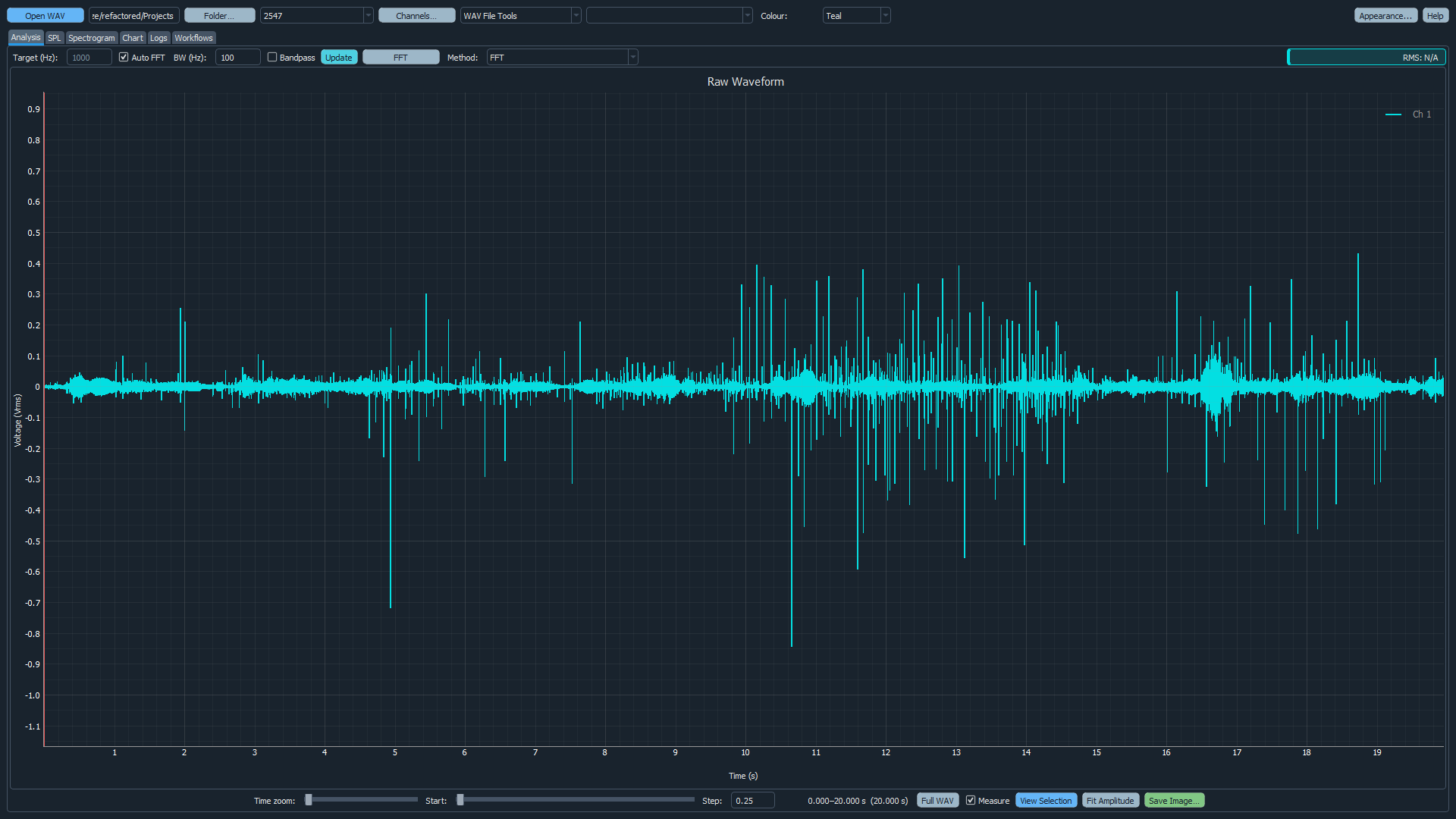
- Inspect the waveform for clipping. Open FFT, select a signal window, and identify the dolphin click or whistle frequency band.
- Set Target Frequency and Bandwidth. Leave Bandpass off unless filtering is part of the documented method.
- Enable Measure and drag across the event, or use the appropriate repeated-event measurement tool.
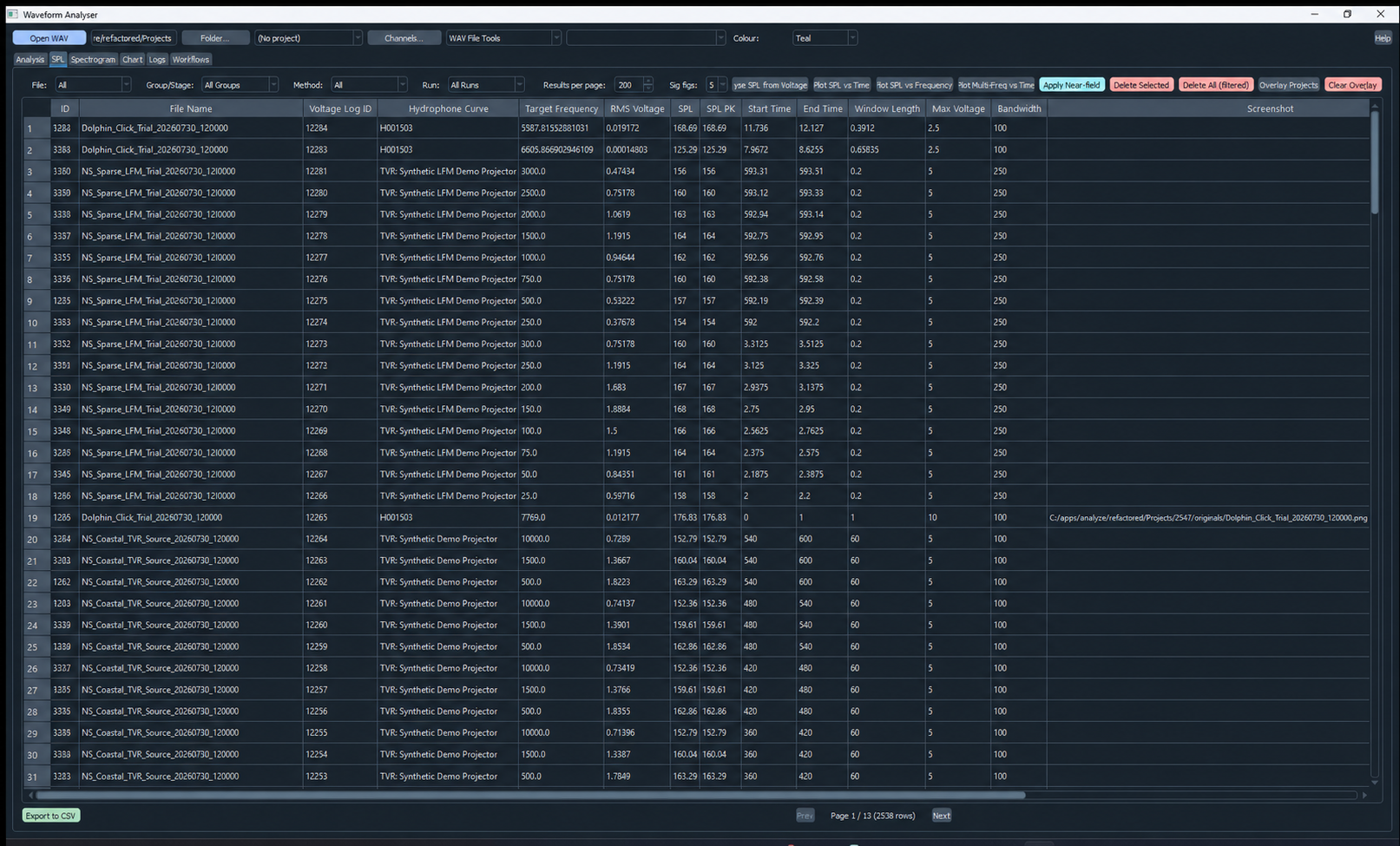
- Open SPL, filter by project/file/method, then choose Plot and inspect SPL vs Time.
- Export the filtered data and retain the channel, sensitivity curve, voltage convention, band, time bounds, distance, and filter state.
Calibration check: a hydrophone sensitivity curve converts received voltage to pressure. A transmitter TVR curve is not a hydrophone curve, and normalised audio cannot support absolute SPL without recoverable physical scaling.
Workflow 03
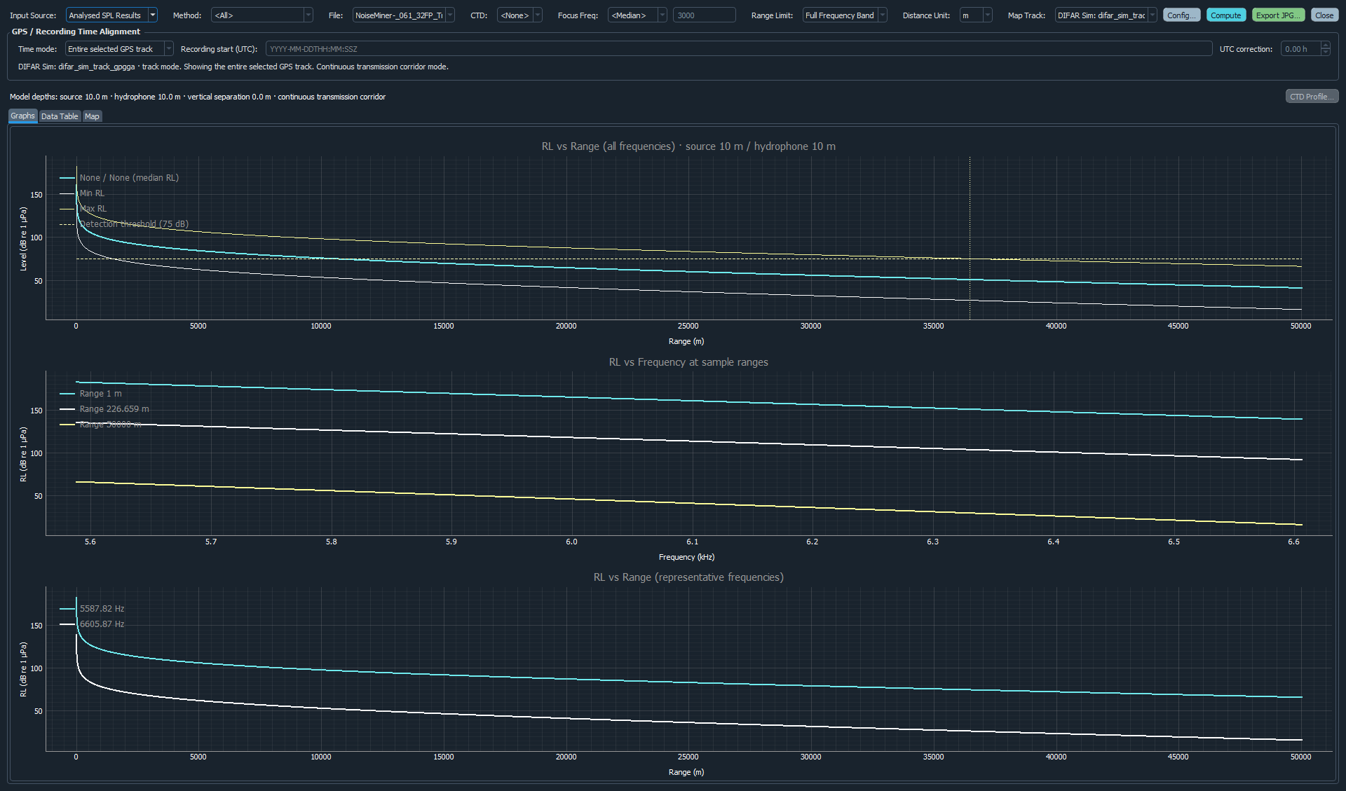
Plan propagation for a sound-source sea trial.
Result: documented scenario curves, tabular outputs, and a mapped planned propagation corridor.
- Create the trial project. Import the planned GPS track, pinger/station positions, bathymetry, and a representative CTD cast when available.
- Prepare source levels: use a TVR curve plus planned drive voltage, or enter a Frequency / SPL table. Confirm dB re 1 µPa @ 1 m.
- Open Modelling & Plotting Tools → Propagation Modelling and choose the planning input source.
- In Config, set source/receiver depths, range grid, spreading, absorption, minimum receive level, sea states, bottom types, and CTD.
- Choose Full Frequency Band for multiple tones or LFM; use Focus Frequency only when one frequency is the decision basis.
- Select the planned track. Use Continuous for a moving source or Discrete with planned timestamps for sparse pings.
- Compute and compare curves, the environment-filtered Data Table, legends, and first 0 dB crossing.
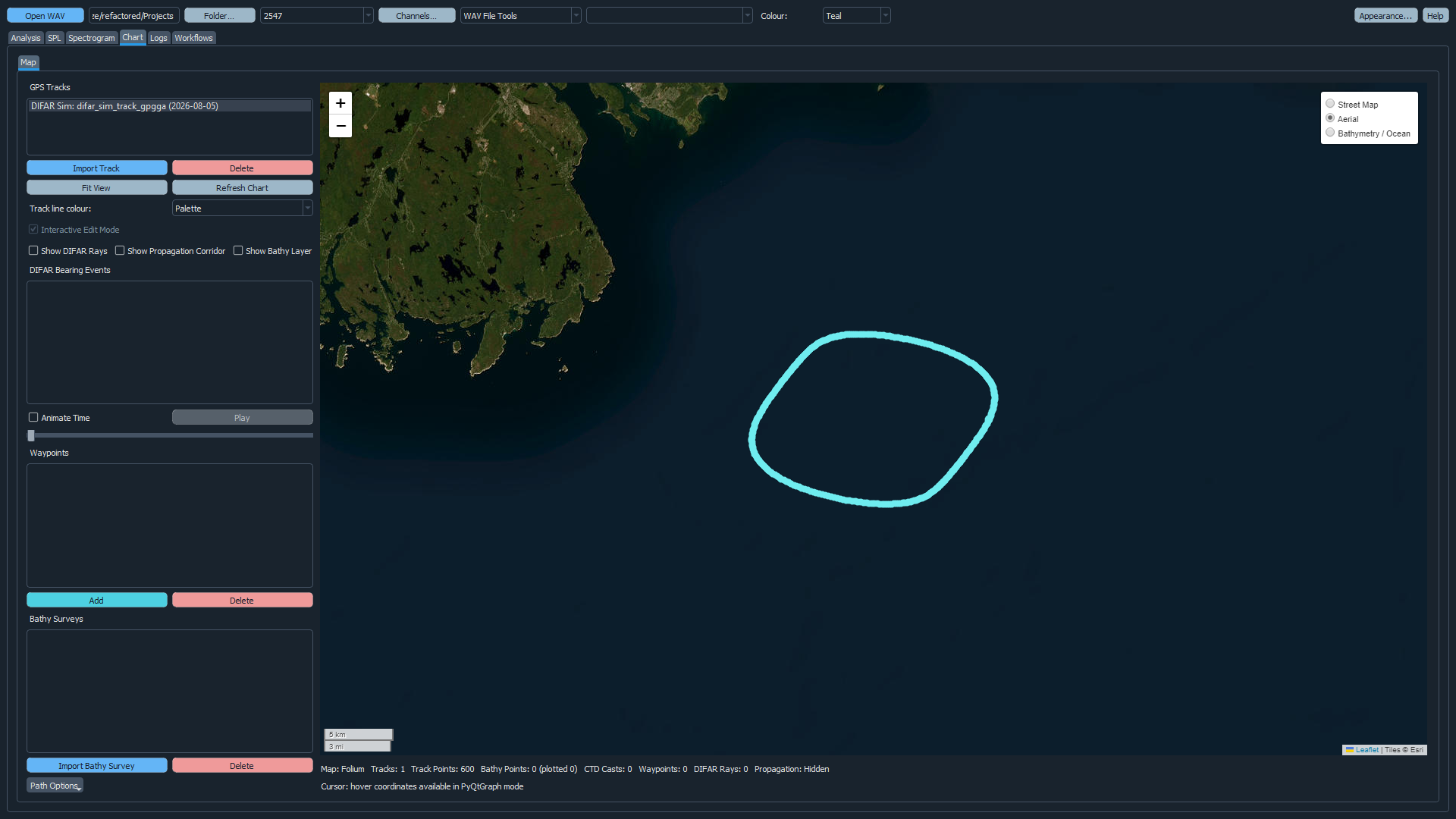
- Review the Map tab, send it to Chart, and check bends, station timing, depths, and ping positions.
- Export the workbook and graph to propagation_model, preserving one worksheet per sea-state/bottom combination and every assumption.
- After the trial, rerun with measured source levels, actual GPS times, deployed depths, and the applicable CTD profile.
Planning limit: this is an engineering screening model. Directivity, bathymetry, surface and seabed conditions, CTD variability, vessel motion, self-noise, and detector performance can change achieved range.
Explore the methods