
GPS tracks
Match analysed files or time-varying source levels to a vessel track.
Sound in operational context
Build propagation cases from analysed recordings, SPL results or entered frequency-level tables, then compare environmental scenarios and detection ranges.
Request a modelling demonstration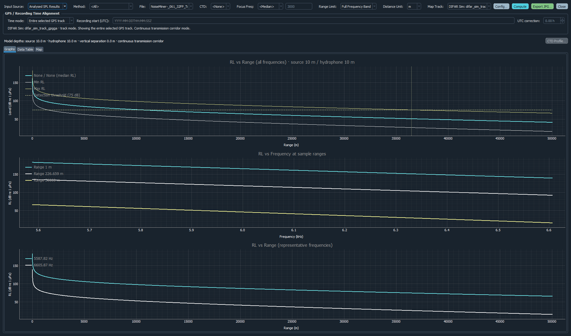
Model inputs
Propagation modelling can begin from a recording analysis, an existing SPL result or a table of SPL and frequency values. This accommodates received hydrophone data as well as source levels derived from voltage measurements and a transmitting-voltage-response curve.
Display range can follow a focus frequency or the complete set of analysed median frequencies, which matters when multiple bands produce materially different ranges.
Select bottom types and sea states as comparison scenarios, filter the displayed results and export each combination in an organised workbook or CSV structure.
Apply a minimum receive level so the table and graph distinguish detectable and non-detectable range points.
Map and water column
Match analysed files or time-varying source levels to a vessel track.
Represent stationary pingers or receivers at project positions.
Display separated pings in time rather than implying continuous transmission.
Preserve changing source or receive levels between transmitted pulses.
Use imported water-column profiles as environmental context for deployment review.
Compare recommended deployment depth with the depths actually used.
Bring the SPL, frequency, timing, positions, depths and CTD profile available for your project.